StarPower:
Getting the most out of product rating scales
★★★★★
Prepared for The Data Incubator Fellowship challenge, February 2017
1. INTRODUCTION AND RATIONALE
Product rating systems from a scale of 1 to k (with k = 5 being most common) are ubiquitous, from Airbnb to Zappos. Typically, ratings are summarized as two statistics: the arithmetic mean, and the number of ratings which comprise it. For example, consider these three products (or any three things that could be rated):
Product A: 10 ratings, mean rating = 4.4
Product B: 100 ratings, mean rating = 4.2
Product C: 1000 ratings, mean rating = 4.0
Product B: 100 ratings, mean rating = 4.2
Product C: 1000 ratings, mean rating = 4.0
All else being equal (price, location, etc.), which product has the “best” rating? Currently, a user’s intuition is the only thing at his or her disposal. This project is designed to help move users from intuition to inference.
Just to keep things simple, let’s assume that the ratings we do have come from valid reviews; that is, we’ve eliminated incentivized reviews, bot reviews, unverified purchases, and so on. Cleaning up a set of reviews is itself a nontrivial problem, and solutions for it have been proposed both in the scholarly literature and via websites like FakeSpot, ReviewMeta, and Trustwerty. But even after eliminating suspicious reviews (and their associated star ratings), two questions remain: (1) What is a useful product-level summary statistic?, and (2) How can this product be ranked or compared against other products?
Just to keep things simple, let’s assume that the ratings we do have come from valid reviews; that is, we’ve eliminated incentivized reviews, bot reviews, unverified purchases, and so on. Cleaning up a set of reviews is itself a nontrivial problem, and solutions for it have been proposed both in the scholarly literature and via websites like FakeSpot, ReviewMeta, and Trustwerty. But even after eliminating suspicious reviews (and their associated star ratings), two questions remain: (1) What is a useful product-level summary statistic?, and (2) How can this product be ranked or compared against other products?
2. TECHNICAL SUMMARY
This project defines a new method of “scoring” a set of product ratings on a 1-to-5 scale, creating an improved method of ranking products which match a set of query conditions. It is divided it into two phases; Phase 1 is complete, with code available here. In my time at The Data Incubator, I hope to bring Phase 2 to fruition.
Phase 1: Back-end analysis
- Gather a large set of 5-level ratings on products from three publically available datasets: Julian McAuley’s Amazon dataset, the Netflix Prize dataset, and the Yelp dataset challenge.
- Tabulate the ratings counts for each unique product.
- Transform these counts into a single weighted score ranging from 0 to 1.
- For each data set (or specific subset of data such as “Books,” “Electronics,” etc.) use empirical Bayes estimation to create a conjugate prior probability distribution: Beta(α,ꞵ).
- Confirm that this method works successfully for all available datasets, ensuring future generalizability.
Phase 2: Front-end deployment
- For a given user query via amazon.com, pull all matching product ASINs and their rating data using the product API.
- For each product, compute the weighted score S using its current ratings data (N total ratings).
- Use the previously derived Beta parameters and Bayesian logic to compute the updated score for each product: (S ∙ N + α) / (N + α + ꞵ).
- Rank the products by their updated score from highest to lowest.
- Return this ranked list to the user.
3. BACK-END ANALYSIS
3.1. The problem with means
Despite their near-universal usage as a summary score for k-level rating scales, means (arithmetic or otherwise) are a non-optimal statistic for two reasons.
First, since rating scales are ordinal by nature, taking the mean (or statistics which derive from it, like the standard deviation or the standard error) is technically inappropriate.
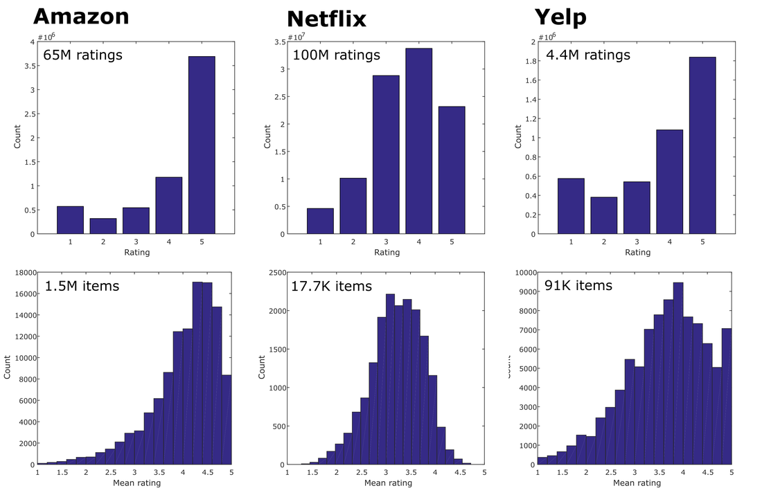
Second, observed distributions of product ratings non-normal, as illustrated in Figure 1. As a result, observed means tend to fall closer to 4.0 stars than 3.0 stars, as would be expected if ratings were normally distributed. Although this phenomenon is well-known to scholars and data scientists, the casual consumer may be completely unaware that the typical rating on Amazon (and elsewhere) is a full “point” off from the scale’s center.
3.2. From means to scores
Instead, it is proposed to multiply a set of ratings counts c = {c1, c2, c3, c4, c5} by a vector of weights w = {w1, w2, w3, w4, w5}, yielding a single summary score: S = c ∙ w.
The value of each weight ranges from 0 to 1, and may be interpreted as follows: “The weight for a given rating level is the hypothesized proportion of raters whose overall opinion of the product was positive.”
For example, a w = {0, .01, .2, .5, 1} would reflect that 50% of raters who give a rating of “4” had a positive opinion of the product, whereas only 1% of raters who gave a rating of “2” did.
Consider how this approach helps solve another potential issue with a mean-based ratings summary. Let’s say we have three products, each 100 ratings, as follows:
Product A: c = {5, 25, 40, 25, 5}
Product B: c = {20, 20, 20, 20, 20}
Product C: c = {36, 12, 4, 12, 36}
Product B: c = {20, 20, 20, 20, 20}
Product C: c = {36, 12, 4, 12, 36}
These three sets of ratings have the same mean: 3.0. However, they have markedly different S values: 0.257, 0.342, and 0.429, respectively. This highlights the potential sensitivity of scores (over that of means) to distinguish products.
This w described here is only a first pass. Weight values could, in fact, be derived rather than chosen arbitrarily. For example, given the set of review texts that were associated with a given rating level (1 to 5), the w value for that rating level could be defined as the proportion texts that were classified as "positive" using sentiment analysis.
This w described here is only a first pass. Weight values could, in fact, be derived rather than chosen arbitrarily. For example, given the set of review texts that were associated with a given rating level (1 to 5), the w value for that rating level could be defined as the proportion texts that were classified as "positive" using sentiment analysis.
3.3. Deriving a conjugate prior distribution using empirical Bayes
Next, a conjugate prior probability density function (PDF) is derived for each dataset by computing the maximum likelihood estimates of the beta distribution parameters α and β from the set of observed S values from that dataset. (S = 0.0 and S = 1.0 values are ignored during this step to avoid model-fitting errors.)
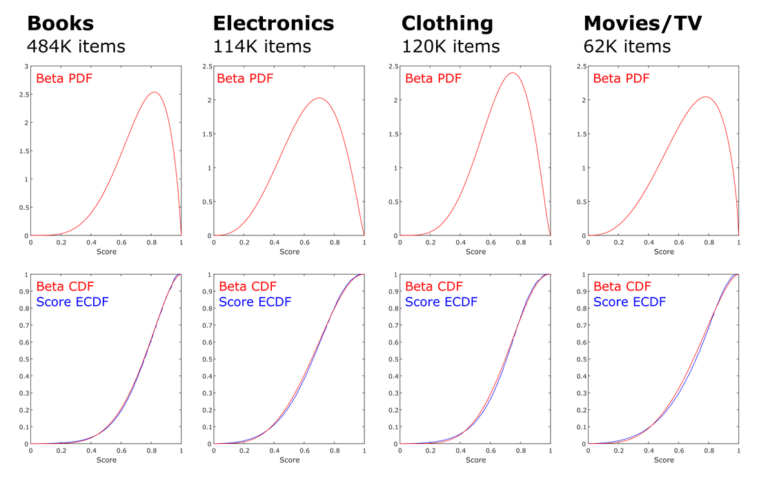
Because the datasets are large, the resultant model fits are very good. As an illustration, Figure 2 presents the empirical cumulative distribution function (ECDF, in blue) for product S values (using w = {0, .01, .2, .5, 1}) in the four largest Amazon subsets, with the PDF of the modeled Beta distributed superimposed in red.
Because the datasets are large, the resultant model fits are very good. As an illustration, Figure 2 presents the empirical cumulative distribution function (ECDF, in blue) for product S values (using w = {0, .01, .2, .5, 1}) in the four largest Amazon subsets, with the PDF of the modeled Beta distributed superimposed in red.
3.4. Updating scores via the relevant conjugate prior
Having obtained a conjugate prior that is specific to each dataset, we can now update our estimate of each product’s S value. Given the beta distribution parameters α and ꞵ, the observed S value, and the number of total ratings N, the updated S is computationally simple:
(S ∙ N + α) / (N + α + ꞵ)
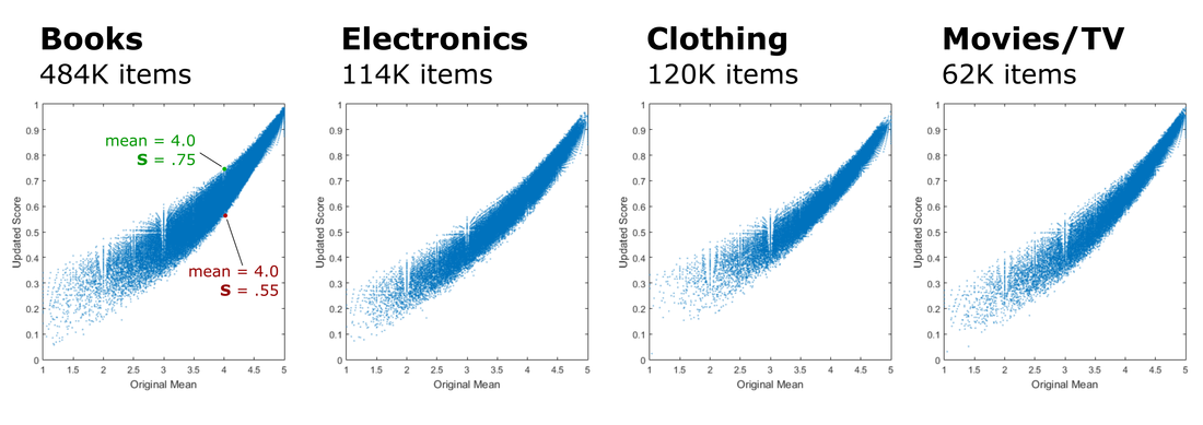
Figure 3 shows the relationship between each product’s mean rating and the updated scores. Although there is a clear relationship between the two variables, it’s the details that matter. For example, the left plot of Figure 3 highlights two books, both with a mean rating = 4.0, but updated S values of .75 and .55, respectively. An S = .75 is in the 76th percentile across all books, whereas S = .55 is only in the 24th percentile. This illustrates the potential for large shifts in product rankings.
4. FRONT-END DEPLOYMENT
Phase 2 of this project is to make it a viable consumer-facing application. To keep the scope manageable, I will focus solely on implementing this approach in the context of amazon.com.
One benefit of the proposed method is that it is lightweight. The “heavy lifting” of deriving the appropriate conjugate prior distribution for a given dataset (with as much granularity as is needed) and refining the estimates of α and ꞵ does not need to be performed in real time.
Ranking products matching a user's query by their Bayesian-updated score offers advantages over a previously suggested approach: ranking products using lower bound of the Wilson score confidence interval (i.e., a frequentist interpretation).
More importantly, the method enables the full power of Bayesian inference to be utilized in the context of understanding differences between product ratings. For example, we could directly compute the probability that the expected value of Product A's score is greater than the expected value of Product B's score by computing the difference between their posterior distributions.
5. GENERALIZABILITY
This method could be applied to any product service which utilizes a k-level rating scale: for example, 2-level scales (Reddit, YouTube), other 5-level scales (BestBuy, Ebay, Glassdoor, OpenTable, TripAdvisor, Udemy), or 10-level scales (Booking.com, FourSquare.com, IMDb.com). As such, I believe that this project would have a broad appeal to potential employers, thus satisfying an important component of what The Data Incubator views as a viable capstone project.


